
Google BigQuery Analytics – ROW_NUMBER

I can teach you analytics! BigQuery is built for analytics, and this week, I will show you row_number, a not-so-distant cousin to rank. I used to think that the row_number analytic was harmless and somewhat useless, and boy, was I wrong. The row_number is one of my favorite analytics, and I will show you many ways to pinpoint specific rows in a dataset, such as the first or last sale per product or the highest or lowest grade point. Get ready to add to your analytic arsenal.
All of these examples have come from my books and training classes. Please do me a favor and tell your training coordinator that you know the best technical trainer in the World. Ask them to hire me to train at your company, either on-site or with a virtual class. They can see our classes, outlines, and a sample of my teaching at this link on our website. I hope to meet you and say thanks in my next class at your company:)
https://coffingdw.com/education/
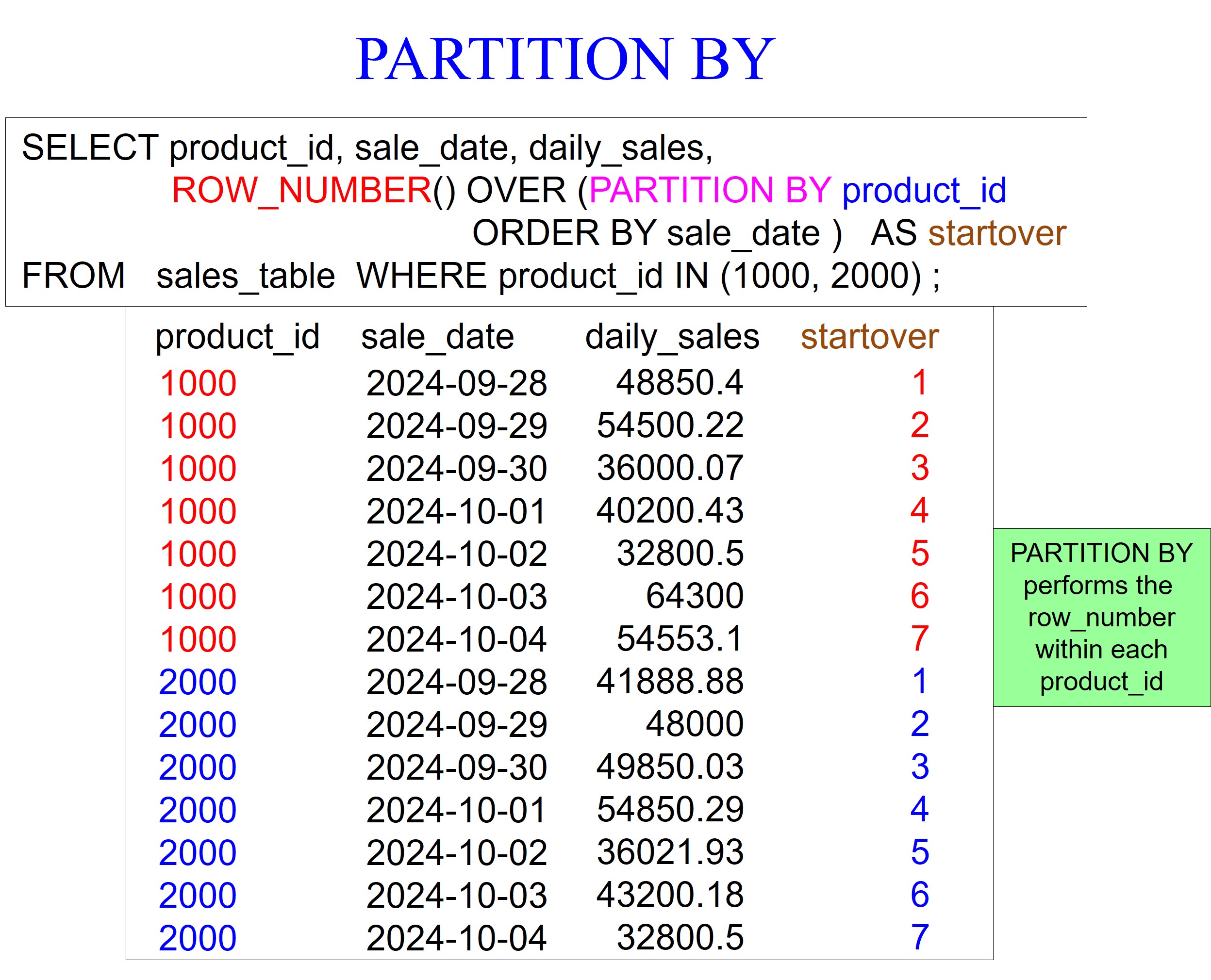
In the picture below, you can see the analytic row_number followed by parenthesis. There is never anything inside the parenthesis, but it signifies that it is a function. You will always have the keyword OVER because before the row_number performs, the dataset will order the data as the ORDER BY statement instructs.
Our example below first orders the data by a major sort of product_id and then a minor sort of sale_date. Notice we see in the result set the product_id of 1000 and within 1000 sequential dates in order. Only after the data is ordered does the row_number place a number starting from one on the first row and incrementing by one until the last. These types of analytics are often referred to as ordered analytics because they order the data before the analytics runs.

Our next example uses a PARTITION BY statement, which means performing the analytic within each product_id separately. I like to think of it as resetting the row_number with the beginning of each product_id. Notice that we are ordering the data by sale_date, but it appears we are ordering by product_id and then sale_date because of the combination of partitioning and ordering within the row_number analytic.
Our example returns the last three sales per product_id, demonstrating the QUALIFY statement’s power. Qualify filters like a WHERE clause, but there is a big difference. A WHERE clause removes rows before a calculation, so the data must exist inside the table. However, a QUALIFY statement filters after the analytic runs. QUALIFY is to analytics what HAVING is to aggregation.
In our example below, we partition by the product_id, and ORDER BY product_id, and sale_date. We didn’t need the product_id repeated in the order by statement, but it won’t hurt us. Notice we are ordering by sale_date in descending order.
We control three things below:
We control it by resetting the row_number calculation using the PARTITION BY PRODUCT_ID statement.
We control how the data will be sorted, which happens to be the sale_date in descending order.
Using the QUALIFY statement, We control how many rows will return per product_id.
I have also placed an ORDER BY statement at the end of the query to ensure the data is presented as I want.

The examples above and below do the same thing, but we are using a brilliant technique I want you to know about. The example below does not return the row_number. Instead of using the row_number analytic in the SELECT list, like in the example above, we use it within the QUALIFY statement below. We still get the last three sales per product_id without having the row_number as part of our answer set.

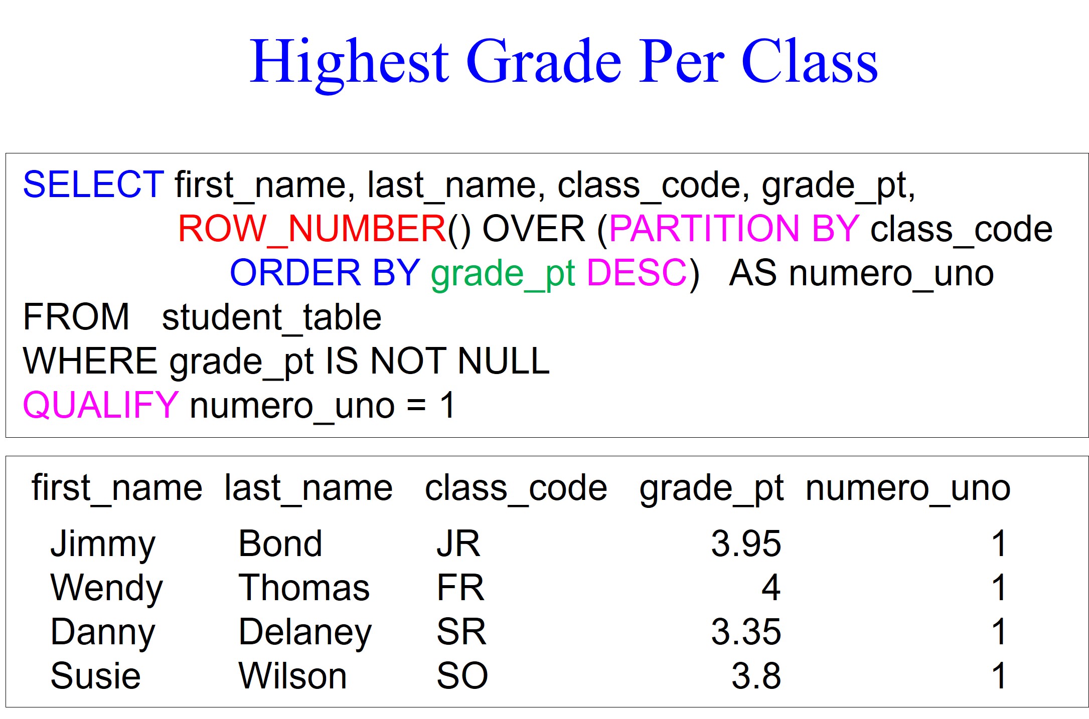
Now that you know what to look for, the example below should be easy on your brain and eyes. We partition by the class_code and order by the grade_pt in descending order. We also use a WHERE clause to filter out grade_pt null values. We use the qualify statement to only return individuals with the highest grade_pt average in their class_code.
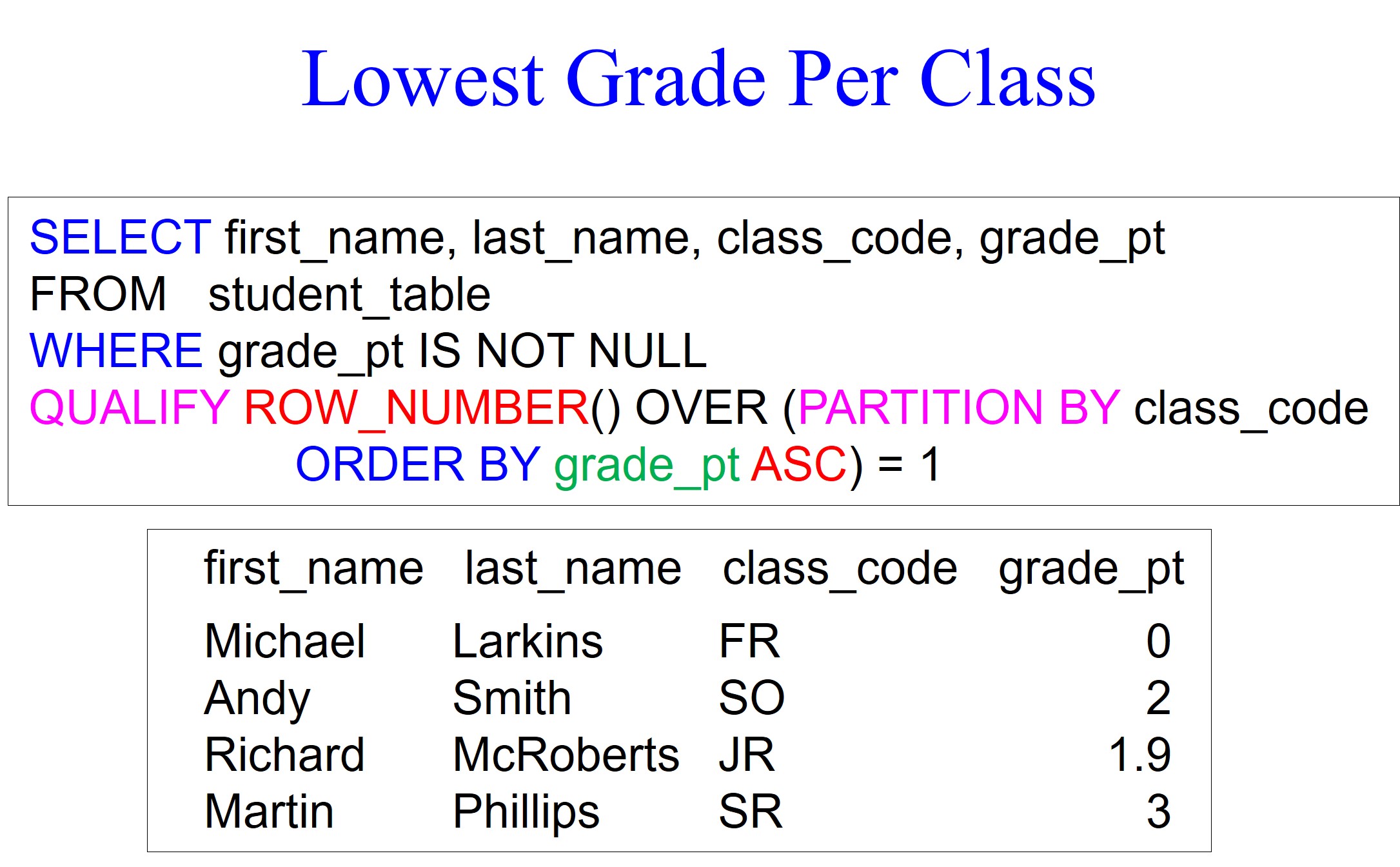
We have made a few changes in our example below to return the lowest grade averages per class_code. We use the qualify statement at the bottom of the query, which partitions by class_code and then orders by grade_pt in ascending order. We get the lowest grade averages per class_code, but without seeing the row_number on the report.
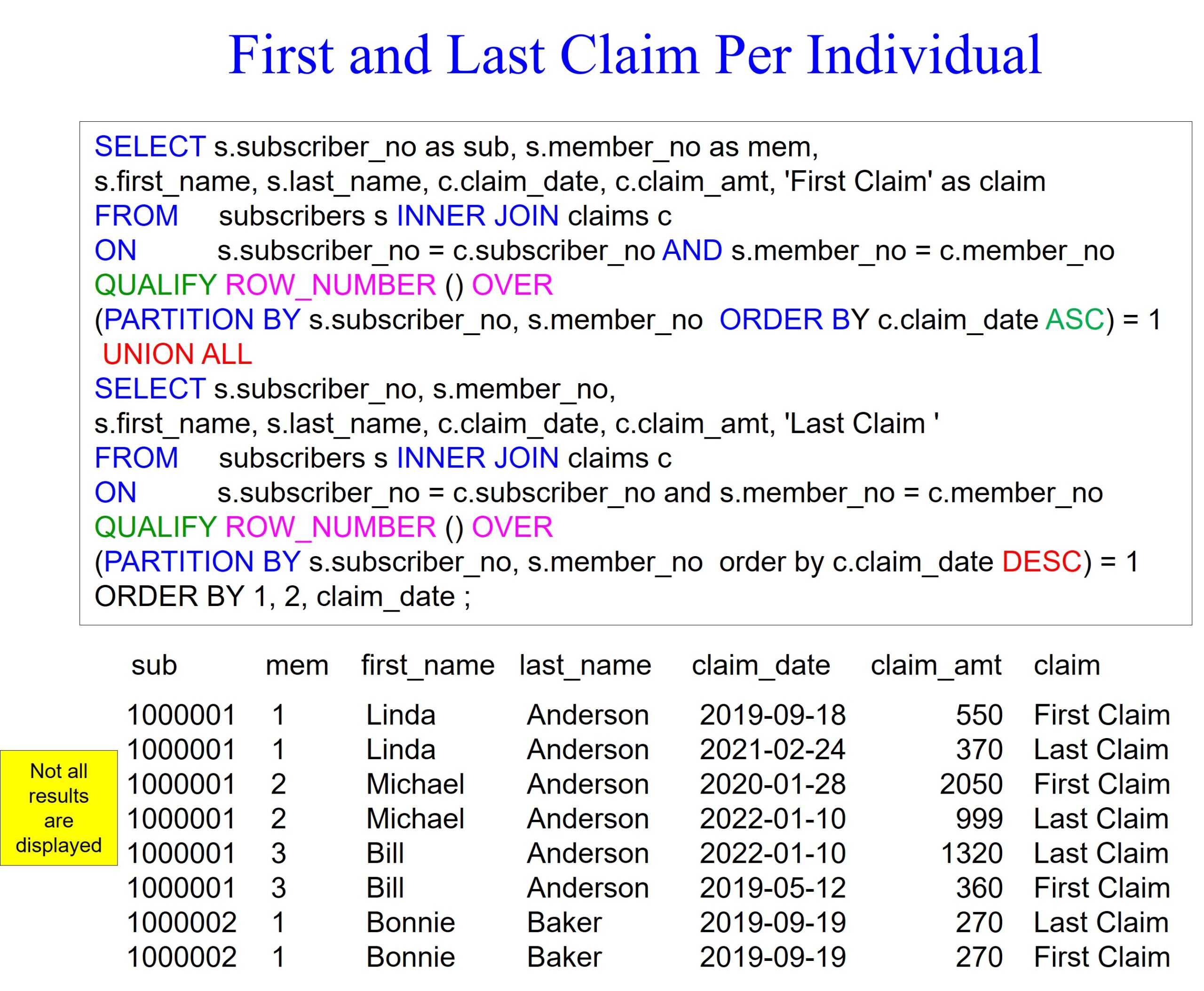
The example below uses clever techniques to find the first and last claim filed per individual. The first thing to focus on is the UNION set operator. A set operator will have two select statements, each with the same amount of columns and similar data types, often referred to as being from the same domain.
We perform a join between the subscribers and claims tables in the top and bottom queries. We also use a QUALIFY statement in both queries and the row_number analytic. We are using two columns in the PARTITION BY statement, which are subscriber_no and member_no because they make up an individual with a policy.
We also order the top query by claim_date asc and the bottom query by claim_date desc. The only other trick is we use the literal ‘First Claim’ in the top query but use the ‘Last Claim ‘ in the bottom query. I purposely put an extra space in ‘Last Claim ‘ to ensure both were the same length.
We now see the first and last claims per individual in our report.
Did you know that Coffing Data Warehousing was the first to create software that joins data across all systems? Download your free Nexus trial at www.CoffingDW.com.
Watch how Nexus performs federated queries to join a BigQuery table to tables from twenty systems in a single query. Watch the video.
To find out more about Nexus, you can watch our 60-second videos here: