
Amazon Redshift Analytics – CUME_DIST

I can teach you analytics! Amazon Redshift is built for analytics, and this week, I will show you CUME_DIST, a not-so-distant cousin to RANK. You can now unlock the power of data insights and uncover hidden trends by mastering CUME_DIST, a vital statistical tool that reveals your dataset’s cumulative distribution of values.
All of these examples have come from my books and training classes. Please do me a favor and tell your training coordinator that you know the best technical trainer in the World. Ask them to hire me to train at your company, either on-site or with a virtual class. They can see our classes, outlines, and a sample of my teaching at this link on our website. I hope to meet you and say thanks in my next class at your company:)
https://coffingdw.com/education/
The CUME_DIST function is an SQL analytic window function that calculates the cumulative distribution of a value within a group of values. CUME_DIST provides a straightforward way of analyzing sales distribution across different products.
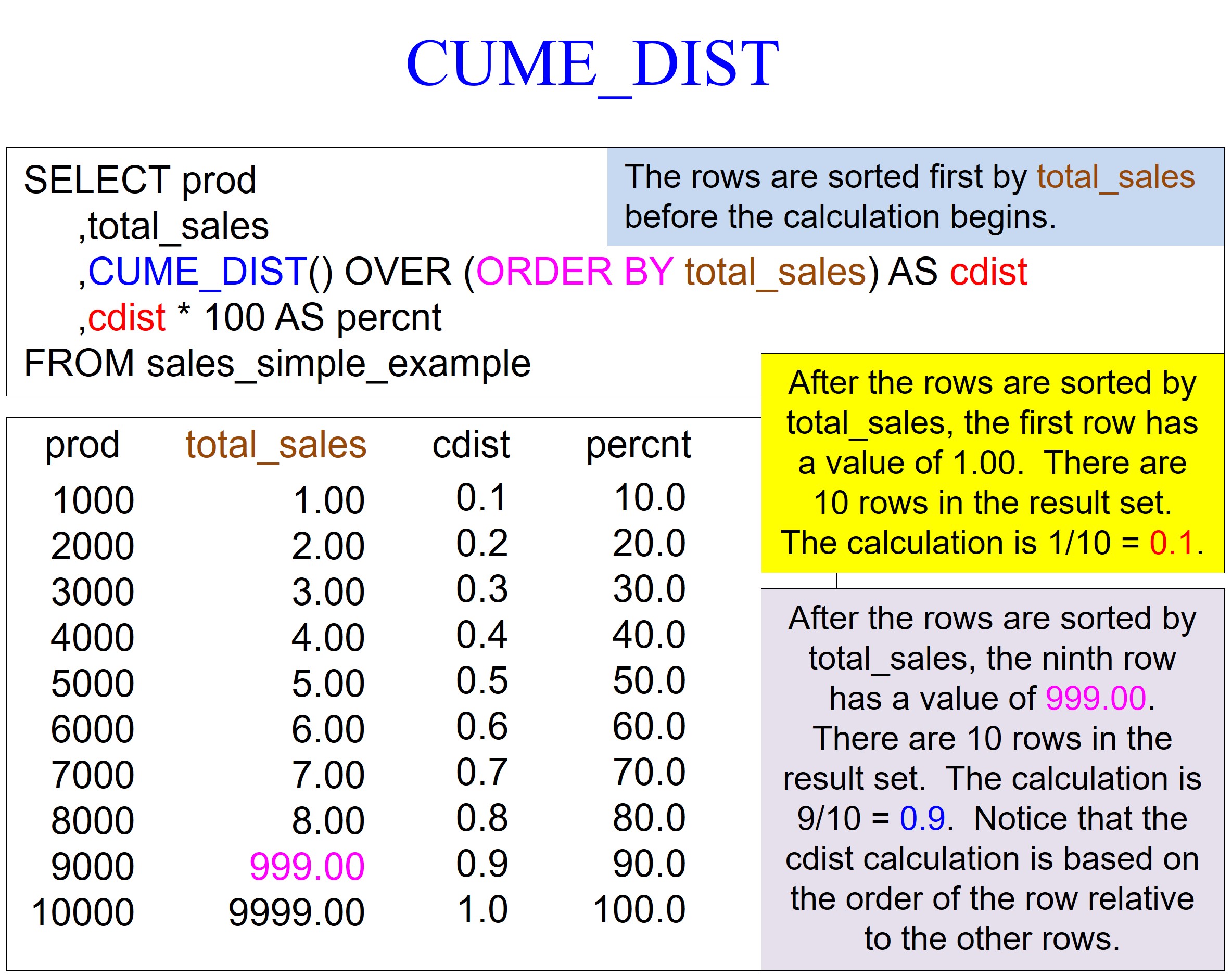
In the picture below, please notice the CUME_DIST followed by the open and closing parenthesis. Nothing is inside the parenthesis, but this signals that CUME_DIST is a function.
You will always have the keyword OVER, meaning the system will perform the CUME_DIST function on an ordered set of values. So before the CUME_DIST function is performed, the system will use the ORDER BY total_sales statement to sort the rows by total_sales. The default of an ORDER BY is ascending mode, which is how the data is sorted.
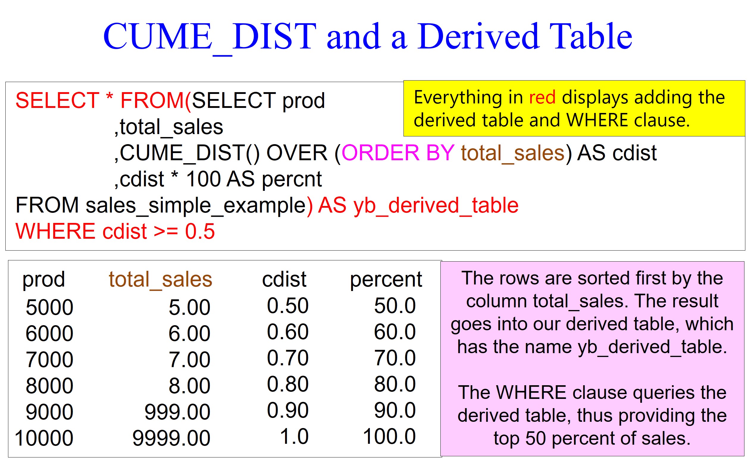
Notice the values I put in the table. The values begin with 1.00 and then 2.00, etc.; I want to keep the values relatively small until we jump to 999.00 and 9999.00. I am demonstrating that CUME_DIST doesn’t judge based on much higher values. It merely orders the rows by the ORDER BY statement and then runs a simple calculation based on the ordering of rows.
The result is between 0 and 1, representing the cumulative distribution of the current row’s value within the ordered set of values.
After total_sales sort the rows, the first row has a value of 1.00. There are ten rows in the result set, so the calculation is 1/10 = 0.1.
The ninth row has a value of 999.00. There are ten rows in the result set. The calculation is 9/10 = 0.9. Notice that the CUME_DIST calculation is based on the order of the row relative to the other rows.
We also multiply the cdist alias by 100 to provide a percentage, sometimes making the calculations easier to understand.
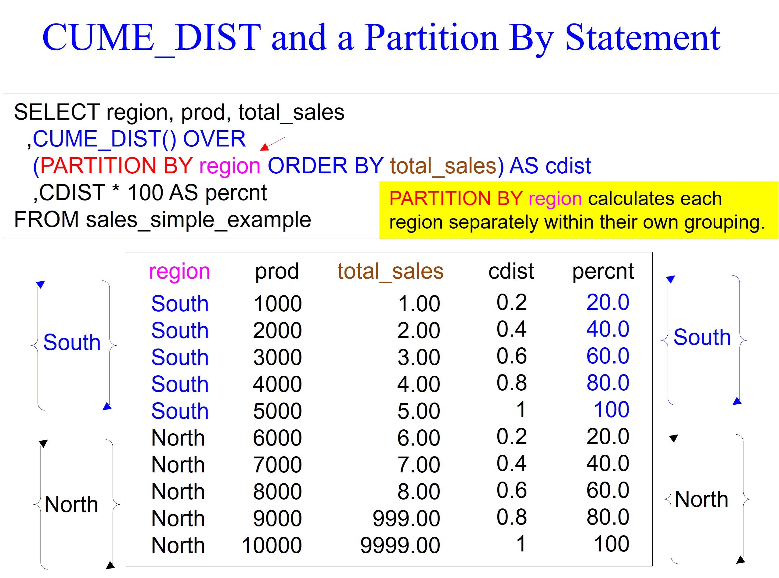
The official definition of CUME_DIST is that the analytic function finds the cumulative distribution of a value with regard to other values within the same window partition.
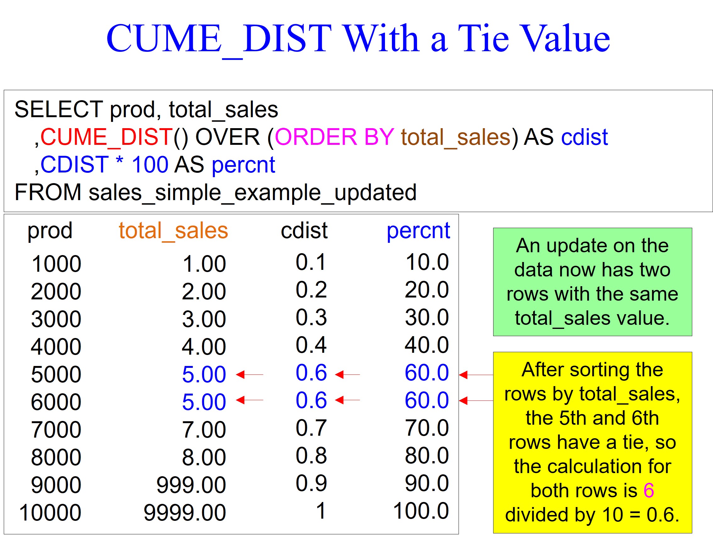
In the example below, we use the PARTITION BY command in column REGION. Since there are two regions, North and South, the CUME_DIST will calculate for only the North region and then reset and calculate the South region.
Even though the total_sales for the North region is vastly higher than the South region, the CUME_DIST calculation is the same. The North and the South regions contain five rows, and once total_sales sorts the rows, the calculations are made not on the total_sales values but on the relative position of the row within its partition.
CUME_DIST is valuable for understanding product sales for many reasons. First of all, it helps to understand market positioning by providing figures of sales in comparison to others. The simplest explanation is that it identifies the high and low performers. How well a product has penetrated a market can also be revealed within a partition such as state, nation, region, etc.
CUME_DIST helps track sales trends over time because it is easy to see if sales are increasing or decreasing, indicating market acceptance or if marketing efforts are paying dividends.
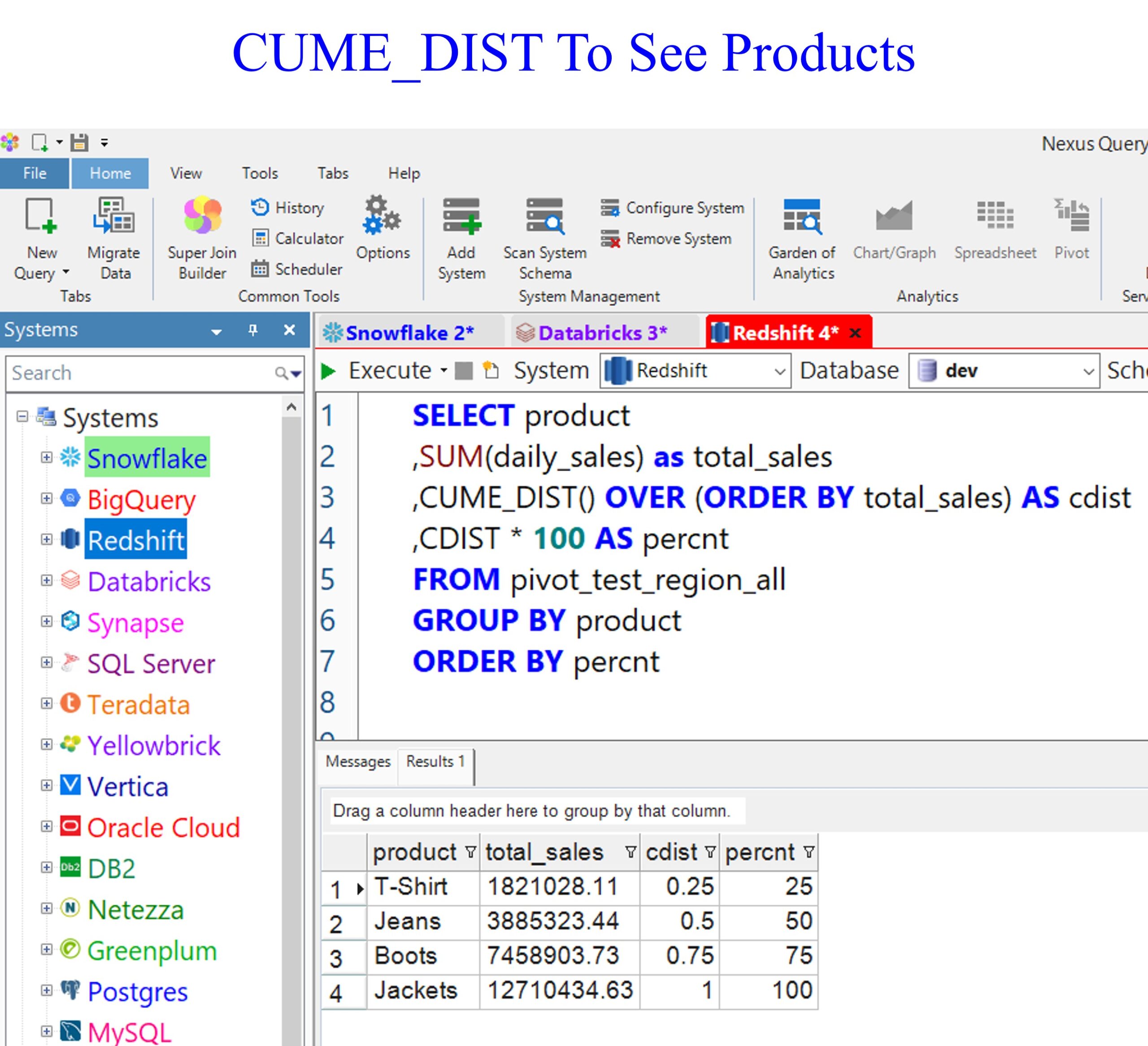
Below is a query that performs a sum of the daily_sales, which we alias total_sales. We then perform a CUME_DIST on the total_sales. Jackets are performing quite well, and T-shirts are our worst performers.
In our example below, we use a derived table to return only rows in the top 50 percent of sales. I have placed everything in red to display what is necessary to add a derived table to use a WHERE clause to filter the rows out with less than the top 50 percent of sales. Because a WHERE clause requires the data you are filtering to already be in a table, we run the query first, place it in a derived table, and then use the WHERE clause to return only the top 50 percent of sales. A derived table only lasts for a single query, and then the system drops it.
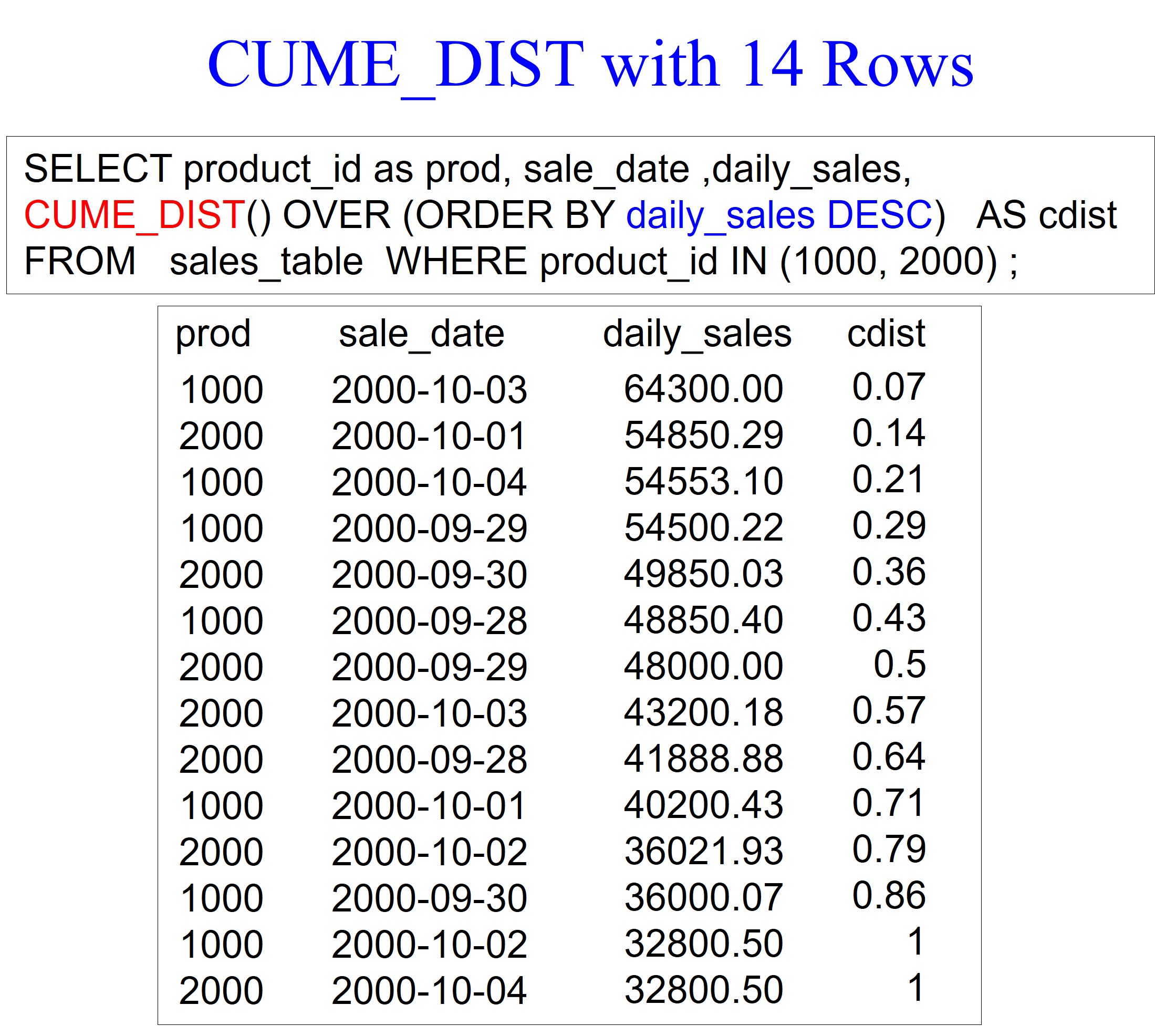
Our example below demonstrates that you can use an ORDER BY in descending mode.
The example shows a CUME_DIST calculation on 14 rows, so the first row after the data is sorted by daily_sales DESC is calculated as one divided by 14, which results in 0.07. The next row is calculated by two divided by 14, which results in 0.14. Notice that rows 13 and 14 have a tie, so they are calculated as 14 divided by 14, which results in one.
Did you know that Coffing Data Warehousing is the first company to create software that joins data across all systems? Download your free Nexus trial at www.CoffingDW.com.
Watch how Nexus performs federated queries to join an Amazon Redshift table to tables from twenty systems in a single query. Watch the video.
To find out more about Nexus, you can watch our 60-second videos here: