
Teradata Analytics – Moving Difference

I can teach you analytics! Teradata is built for analytics, and this week, I will show you the amazing moving difference. The moving difference is one of the most incredible aspects of analytics, but it cannot seem very clear unless it is explained correctly. With power comes incredible responsibility. I won’t disappoint you.
All of these examples have come from my books and training classes. Please do me a favor and tell your training coordinator that you know the best technical trainer in the World. Ask them to hire me to train at your company, either on-site or with a virtual class. They can see our classes, outlines, and a sample of my teaching at this link on our website. I hope to meet you and say thanks in my next class at your company:)
https://coffingdw.com/education/
Moving differences are commonly used in data analysis to understand the rate of change in a series of values over time, which allows us to look for positive or negative trends. They provide insights into the direction and magnitude of change, which can be useful for decision-making and forecasting. Check out the example below.
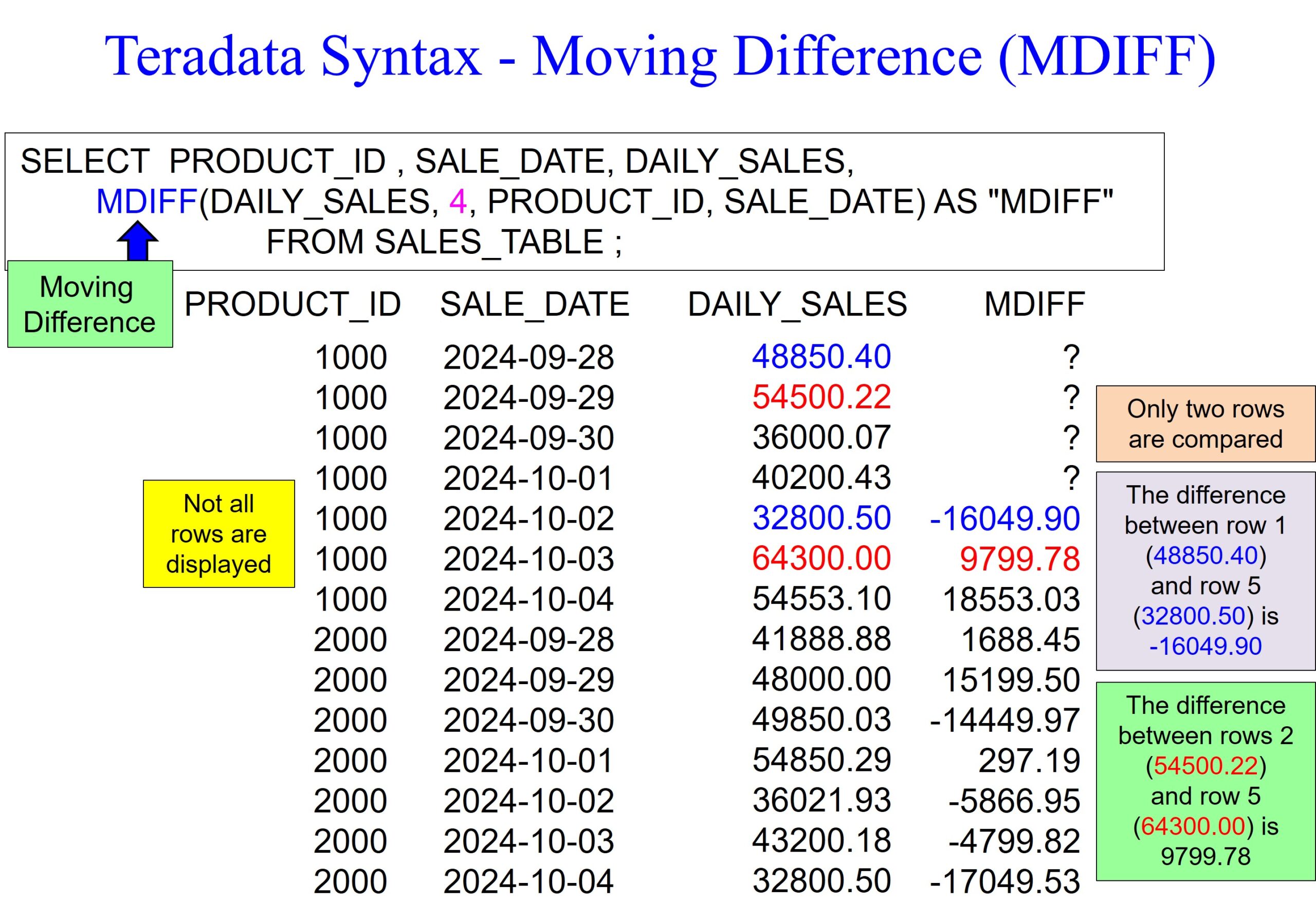
Let me caution you so you are not confused. A moving difference only compares one row to another row. Notice we have an MDIFF(DAILY_SALES, 4), which means to compare the current row’s DAILY_SALES value with the DAILY_SALES value four rows ahead.
I will show you several different syntax options for the moving difference that Teradata uses, and the first is unique to Teradata. Below, you see Teradata’s simplified version of the moving difference. The first thing you see is the MDIFF keyword. Inside the parenthesis, you immediately see the column to perform the MDIFF calculation, which is DAILY_SALES, followed by the moving window of four, which means calculate the difference between the current row’s DAILY_SALES value and compare it with the DAILY_SALES value four rows ahead.
After number four, which is the moving window, you see how to order the data first, with PRODUCT_ID as the major sort and then SALE_DATE as the minor sort.
The first thing to remember is that these analytics are often referred to as ORDERED ANALYTICS because they order the data first and then perform the calculation. Once the data is ordered correctly, the analytic calculates from the first row sorted to the last. In our example below, we first order from PRODUCT_ID and then SALE_DATE.
If I have a moving window of four, as in the example below, then the DAILY_SALES of row one will compare to the DAILY_SALES value of row five (four rows apart) and show a positive or negative difference between those two rows.
Notice that the first four rows have null values in the moving difference. Why? Because each of them has something in common: they don’t have a row four rows ahead of them to compare.
Notice that the fifth row has a value of -16409.90. We are only comparing the DAILY_SALES value in row one with the DAILY_SALES value in row five because we have a moving window of four. I have colored those values in blue. Notice that we compared row two with row six (four rows apart), and we did better by 9,799.78 dollars, colored in red.
The example below performs the same moving difference calculation every four rows but uses the LAG command. Remember, both examples only compare the difference between the current row’s daily_sales and the daily_sales value four rows ahead.
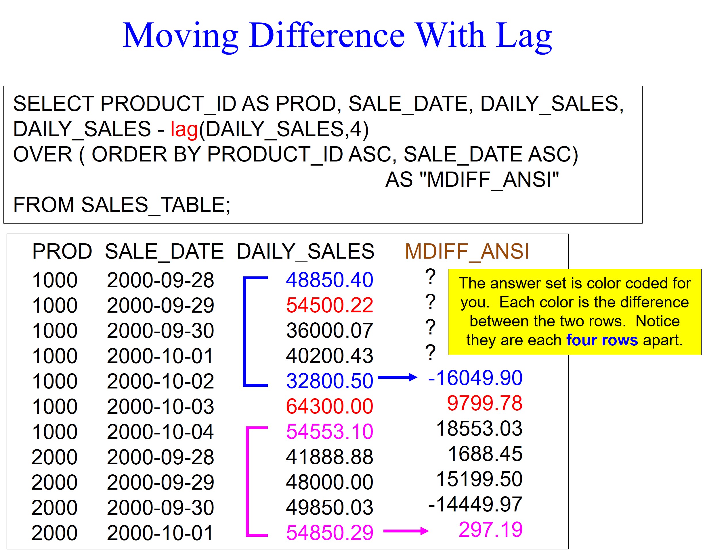
In the picture below, notice that we have a GROUP PRODUCT_ID before our ORDER BY statement. The keywords GROUP BY mean only to perform the calculation within each PRODUCT_ID. Within each PRODUCT_ID, we order the data by SALE_DATE.
Also, notice that we have a moving window of four rows because of the number four inside the MDIFF calculation.
The moving difference calculation below will compare the DAILY_SALES value of the current row with the DAILY_SALES value four rows before. Remember, only two rows are compared, so we are comparing rows one and five for a moving difference of -16,049.90. In other words, we had a DAILY_SALES value of $48850.40 in row one. When we compared $48,850.40 with row five’s value of $32,800.50, we did worse by 16,049.90. Ouch!
Also, notice that we had null values for the first four rows in each PRODUCT_ID grouping because there were not any rows four rows ahead.

The example below is the best way to learn a Teradata moving difference because it uses ANSI syntax, meaning it will work on every database. The ANSI syntax is a little harder to understand initially, but it eventually becomes easy.
The first thing to remember is that these analytics are often referred to as ORDERED ANALYTICS because we have an ORDER BY statement inside the calculation that sorts the data first. Once the data is ordered correctly, the analytic calculates from the first row sorted to the last. In our example below, we first order from PRODUCT_ID ASC and then SALE_DATE ASC. We don’t need the ASC because ascending mode is the default, but I put it there for clarity.
If I have a moving window of four, as in the example below, then the DAILY_SALES of row one will compare to the DAILY_SALES value of row five (four rows apart) and show a positive or negative difference between those two rows.
Notice that the first four rows have null values in the moving difference. Why? Because each of them has something in common: they don’t have a row four rows ahead of them to compare. Notice that the fifth row has a value of -16409.90. We are only comparing the DAILY_SALES value in row one with the DAILY_SALES value in row five because we have a moving window of four because of the keywords ROWS BETWEEN 4 PRECEDING AND 4 PRECEDING. I have colored those values in blue. Notice that we compared row two with row six (four rows apart), and we did better by 9,799.78 dollars, colored in red.

In the picture below, notice that we have a PARTITION BY PRODUCT_ID before our ORDER BY statement. PARTITION BY replaces our previous example that used GROUP BY, but they do the same thing. The keywords PARTITION BY mean only to perform the calculation within each PRODUCT_ID. Within each PRODUCT_ID, we order the data by SALE_DATE.
Also, notice that we have a moving window of two rows because of the keywords ROWS BETWEEN 2 PRECEDING and 2 PRECEDING.
The moving difference calculation below will compare the DAILY_SALES value of the current row with the DAILY_SALES value two rows before. Remember, only two rows are compared, so we are comparing rows one and three for a moving difference of -12,850.33. In other words, we had a DAILY_SALES value of $48850.40 in row one. When we compared $48,850.40 with row three’s value of $36,000.07, we did worse by 12,850.33. Ouch again!
Also, notice that we had null values for the first two rows in each PRODUCT_ID partition because there were not any rows two rows ahead.

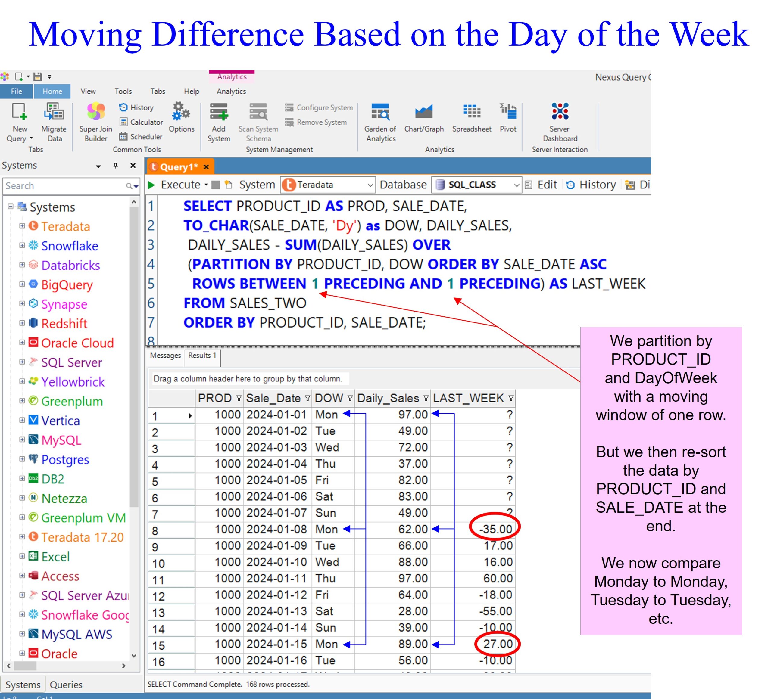
The example below is pure genius and is your ticket to superstar status. We are comparing the DAILY_SALES to what we did the previous week. So, we will compare the DAILY_SALES that happened on a Monday with what happened the previous Monday. And compare Tuesday to Tuesday, etc.
I use several tricks to ensure that this is perfect. The first trick is using the TO_CHAR command to format the SALE_DATE to provide the day of the week, which I alias as DOW. I then PARTITION BY PRODUCT_ID and DOW to calculate the data by PRODUCT_ID 1000, and then all of my Mondays are ordered back to back. These are followed by all of my Tuesdays in a row. I then use a moving window of one because of the keywords ROWS BETWEEN 1 PRECEDING and 1 PRECEDING.
The final trick I use is to put an additional ORDER BY statement at the end of the query where the major sort is PRODUCT_ID, and the minor sort is SALE_DATE.
The moving difference calculation ordered the data by PRODUCT_ID and day of the week. The moving difference calculated Monday to the previous Monday, Tuesday to the previous Tuesday, etc. However, with the addition of the ORDER BY PRODUCT_ID SALE_DATE at the end, I resorted to it to make the report look nice. However, if you compare the first Monday, we made 97.00 to the second Monday, where we made 62.00, we did worse on the second Monday by 35.00. But we did better on the second Tuesday than the first Tuesday by 17.00.
You can also see we compare the third Monday with the second Monday to get a moving difference of 27.00 dollars. Yeah!
Did you know that Coffing Data Warehousing is the first company to create software that joins data across all systems? Download your free Nexus trial at www.CoffingDW.com.
Watch how Nexus performs federated queries to join a Teradata table to tables from twenty systems in a single query. Watch the video.
To find out more about Nexus, you can watch our 60-second videos here: